Simulate data from nested partially-latent class model (npLCM) family

Usage

simulate_nplcm(set_parameter)

Arguments

set_parameter

True model parameters in an npLCM specification:

cause_list: a vector of disease class names among cases (since the causes could be multi-agent (e.g., multiple pathogens may cause an individual case's pneumonia), so its length could be longer than the total number of unique causative agents)
etiology: a vector of proportions that sum to 100 percent
pathogen_BrS: a vector of putative causative agents' names measured in bronze-standard (BrS) data. This function simulates only one slice defined by specimen``test``pathogen
pathogen_SS: a vector of pathogen names measured in silver-standard (SS) data.
meas_nm: a list of specimen``test names e.g., list(MBS = c("NPPCR"),MSS="BCX") for nasopharyngeal (NP) specimen tested by polymerase chain reaction (PCR) - NPPCR and blood (B) tested by culture (Cx) - BCX
Lambda: controls' subclass weights $\nu_1, \nu_2, \ldots, \nu_K$ a vector of K probabilities that sum to 1.
Eta: a matrix of dimension length(cause_list) by K; each row represents a disease class (among cases); the values in that row are subclass weights $\eta_1, \eta_2, \ldots, \eta_K$ for that disease class, so needs to sum to one. In Wu et al. 2016 (JRSS-C), the subclass weights are the same across disease classes across rows. But when simulating data, one can specify rows with distinct subclass weights - it is a matter whether we can recover these parameters (possible when some cases' true disease classes are observed)
PsiBS/PsiSS: False positive rates for Bronze-Standard data and for Silver-Standard data. For example, the rows of PsiBS correspond to the dimension of the particular slice of BrS measures, e.g., 10 for 10 causative agents measured by NPPCR; the columns correspond to K subclasses; generically, the dimension is J by K PsiSS is supposed to be a vector of all zeros (perfect specificity in silver-standard measures).
ThetaBS/ThetaSS: True positive rates $\Theta$ for Bronze-Standard data and for Silver-Standard data. Dimension is J by K (can contain NA if the total number of causative agents measured by BrS or SS exceeds the measured causative agents in SS. For example, in PERCH study, nasopharyngeal polymerase chain reaction (NPPCR; bronze-standard) may target 30 distinct pathogens, but blood culture (BCX; silver-standard) may only target a subset of the 30, so we have to specify NA in ThetaSSfor those pathogens not targeted by BCX).
Nu: the number of control subjects
Nd: the number of case subjects

Value

A list of diagnostic test measurements, true latent statues:

data_nplcm: a list of structured data (see nplcm() for description).
template: a matrix: rows for causes (may comprise a single or multiple causative agents), columns for measurements; generated as a lookup table to match disease-class specific parameters (true and false positive rates)
latent_cat: integer values to indicate the latent category. The integer code corresponds to the order specified in set_parameter$etiology. Controls are coded as length(set_parameter$etiology)+1.)

Examples

K.true  <- 2   # no. of latent subclasses in actual simulation. 
               # If eta = c(1,0), effectively, it is K.true=1.
J       <- 21   # no. of pathogens.
N       <- 600 # no. of cases/controls.

eta <- c(1,0) 
# if it is c(1,0),then it is conditional independence model, and
# only the first column of parameters in PsiBS, ThetaBS matter!

seed_start <- 20150202
print(eta)
#> [1] 1 0

# set fixed simulation sequence:
set.seed(seed_start)

ThetaBS_withNA <- c(.75,rep(c(.75,.75,.75,NA),5))
PsiBS_withNA <- c(.15,rep(c(.05,.05,.05,NA),5))

ThetaSS_withNA <- c(NA,rep(c(0.15,NA,0.15,0.15),5))
PsiSS_withNA <- c(NA,rep(c(0,NA,0,0),5))

set_parameter <- list(
  cause_list      = c(LETTERS[1:J]),
  etiology        = c(c(0.36,0.1,0.1,0.1,0.1,0.05,0.05,0.05,
                 0.05,0.01,0.01,0.01,0.01),rep(0.00,8)), 
                 #same length as cause_list.
  pathogen_BrS    = LETTERS[1:J][!is.na(ThetaBS_withNA)],
  pathogen_SS     = LETTERS[1:J][!is.na(ThetaSS_withNA)],
  meas_nm         = list(MBS = c("MBS1"),MSS="MSS1"),
  Lambda          = eta, #ctrl mix
  Eta             = t(replicate(J,eta)), #case mix, row number equal to Jcause.
  PsiBS           = cbind(PsiBS_withNA[!is.na(PsiBS_withNA)],
                          rep(0,sum(!is.na(PsiBS_withNA)))),
  ThetaBS         = cbind(ThetaBS_withNA[!is.na(ThetaBS_withNA)],
                          rep(0,sum(!is.na(ThetaBS_withNA)))),
  PsiSS           = PsiSS_withNA[!is.na(PsiSS_withNA)],
  ThetaSS         = ThetaSS_withNA[!is.na(ThetaSS_withNA)],
  Nu      =     N, # control size.
  Nd      =     N  # case size.
)
 simu_out <- simulate_nplcm(set_parameter)
 data_nplcm <- simu_out$data_nplcm
 
 pathogen_display <- rev(set_parameter$pathogen_BrS)
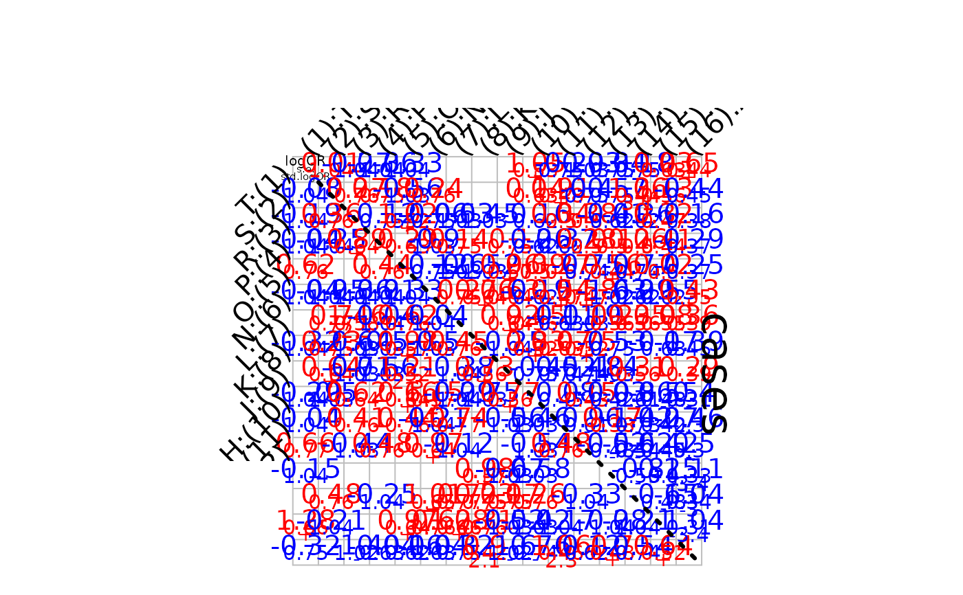
 plot_logORmat(data_nplcm,pathogen_display)
#> == Visualizing pairwise log odds ratios for bronze-standard data set:  1 :  MBS1 . ==

 # more examples are provided in the vignette, including settings with 
 # covariates.

Simulate data from nested partially-latent class model (npLCM) family

Usage

Arguments

Value

See also

Examples